Latest news about Bitcoin and all cryptocurrencies. Your daily crypto news habit.
Many popular apps on both Android and iOS make extensive use of on-device machine learning. Apps like Inbox by Gmail or Siri make use of on device machine learning because it’s faster and does a better job of protecting a user’s privacy. iOS and Android both have proper API support for using on device, neural networks for prediction purposes. On both platforms you can either wire up your own neural network or use a higher level framework like TensorFlow to do the heavy lifting for you.
Tensor & Flow is a two part series where we will explore the specifics of what is needed to do to deploy a machine learning model to an Android app. I will be using TensorFlow Mobile in Part 1, and TensorFlow Lite in Part 2.
 Tensor & Flow demo app on Android
Training a Neural Network
The very first step on this journey is training a neural network that I can deploy. There are plenty of tutorials that walk aspiring machine learning engineers through building models that can classify flowers, identify objects in pictures, detect spam, and even apply filters to pictures. I chose a rather accessible tutorial, building a model to recognize handwritten numbers.
A Guide to TF Layers: Building a Convolutional Neural Network walks us through the entire process configuring and training a neural network to recognize handwritten characters. This guide walks us neural network configuration, downloading the dataset used for training, and the training process.
The first step is configuring our neural network.
The Neural Network
The MNIST tutorial trains a Convolutional Neural Network (CNN) to recognize handwritten numbers.
 Feature extraction using convolution — Source
A CNN is comprised of several different layers:
- Convolutional layers, use convolution operations to extract features from images.
- Pooling layers, down sample the images, which reduces processing time and increases training and inference performance.
- Dense layers, predict a class using the features extracted in the convolutional layers.
Before continuing, I encourage you to make your way over to the Data Science Blog where Ujjwal Karn has written up a very intuitive blog post aptly named “An Intuitive Explanation of Convolutional Neural Networks”. Once you have finished the blog post, visit 2D Visualization of a Convolutional Neural Network for a cool demonstration of a CNN in action.
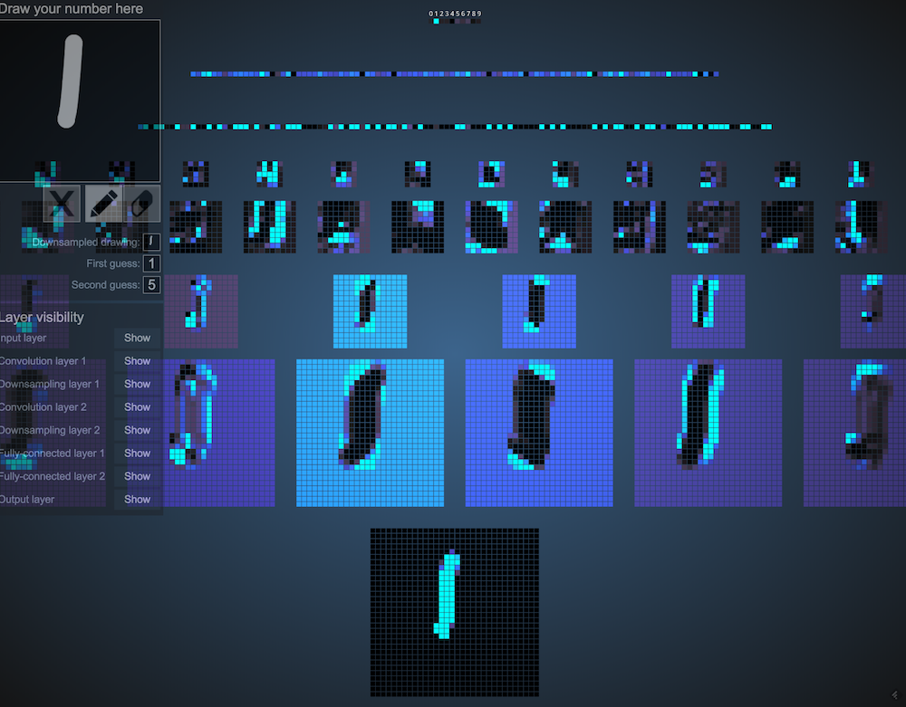 2D Visualization of a CNN
Some more specifics about the neural network in this example, the input layer is a one to one mapping of the size of the input data. The MNIST dataset contains tens of thousands of handwritten number samples and labels. Each sample is a monochrome image of a handwritten digit, 28 pixels x 28 pixels. An image is a 2-dimension array, containing of pixel data, meaning our input layer has 784 input nodes (28 x 28 = 784).
The output layer, a Logits layer, that emits our predictions as raw values. The network uses several additional functions to convert this raw data into a prediction and probability (for training).
Training & Prepping for Integration
The process for training and integrating a neural network model into an Android app resembles:
- Train the neural network.
- Freeze & optimize the TensorFlow graph for inference.
- View the neural network model in TensorBoard. (optional)
- Import the optimized graph into our Android project.
Getting everything setup to do the training can be more difficult than the actual training depending on your computing platform. My setup:
- MacBook Pro (2015) running MacOS 10.13
- IDE: PyCharm, made this easier by auto-importing Python dependencies and providing code debugging capabilities
- Python 2.7.13
- TensorFlow 1.5
- Android Studio 3.0.1
Our guide “A Guide to TF Layers” walks us through setting up our neural network and training. After a few passes through the guide, I made one tweak that made integration into an Android app a bit easier, I gave explicit names to my input and output layers, “input” & “output”, respectively. I did this after spending a few hours attempting to figure out on my own. If you do not name the layers in your neural network, they are given default names. You’ll need to open your trained graph in TensorBoard to determine the names of your layers.
We will end up with this Python script:
from __future__ import absolute_importfrom __future__ import divisionfrom __future__ import print_function
# Importsimport numpy as npimport tensorflow as tf
tf.logging.set_verbosity(tf.logging.INFO)
def cnn_model_fn(features, labels, mode): """Model function for CNN.""" # Input Layer input_layer = tf.reshape(features["x"], [-1, 28, 28, 1], name="input")
# Convolutional Layer #1 conv1 = tf.layers.conv2d( inputs=input_layer, filters=32, kernel_size=[5, 5], padding="same", activation=tf.nn.relu)
# Pooling Layer #1 pool1 = tf.layers.max_pooling2d(inputs=conv1, pool_size=[2, 2], strides=2)
# Convolutional Layer #2 and Pooling Layer #2 conv2 = tf.layers.conv2d( inputs=pool1, filters=64, kernel_size=[5, 5], padding="same", activation=tf.nn.relu) pool2 = tf.layers.max_pooling2d(inputs=conv2, pool_size=[2, 2], strides=2)
# Dense Layer pool2_flat = tf.reshape(pool2, [-1, 7 * 7 * 64]) dense = tf.layers.dense(inputs=pool2_flat, units=1024, activation=tf.nn.relu) dropout = tf.layers.dropout( inputs=dense, rate=0.4, training=mode == tf.estimator.ModeKeys.TRAIN)
# Logits Layer logits = tf.layers.dense(inputs=dropout, units=10)
predictions = { # Generate predictions (for PREDICT and EVAL mode) "classes": tf.argmax(input=logits, axis=1, name="output"), # Add `softmax_tensor` to the graph. It is used for PREDICT and by the # `logging_hook`. "probabilities": tf.nn.softmax(logits, name="softmax_tensor") }if mode == tf.estimator.ModeKeys.PREDICT: return tf.estimator.EstimatorSpec(mode=mode, predictions=predictions)
# Calculate Loss (for both TRAIN and EVAL modes) loss = tf.losses.sparse_softmax_cross_entropy(labels=labels, logits=logits)
# Configure the Training Op (for TRAIN mode) if mode == tf.estimator.ModeKeys.TRAIN: optimizer = tf.train.GradientDescentOptimizer(learning_rate=0.001) train_op = optimizer.minimize( loss=loss, global_step=tf.train.get_global_step()) return tf.estimator.EstimatorSpec(mode=mode, loss=loss, train_op=train_op)
# Add evaluation metrics (for EVAL mode) eval_metric_ops = { "accuracy": tf.metrics.accuracy( labels=labels, predictions=predictions["classes"])} return tf.estimator.EstimatorSpec(mode=mode, loss=loss, eval_metric_ops=eval_metric_ops)def main(unused_argv): # Load training and eval data mnist = tf.contrib.learn.datasets.load_dataset("mnist") train_data = mnist.train.images # Returns np.array train_labels = np.asarray(mnist.train.labels, dtype=np.int32) eval_data = mnist.test.images # Returns np.array eval_labels = np.asarray(mnist.test.labels, dtype=np.int32)# Create the Estimator mnist_classifier = tf.estimator.Estimator(model_fn=cnn_model_fn, model_dir="/tmp/mnist_convnet_model")
# Set up logging for predictions tensors_to_log = {"probabilities": "softmax_tensor"} logging_hook = tf.train.LoggingTensorHook(tensors=tensors_to_log, every_n_iter=50)# Train the model train_input_fn = tf.estimator.inputs.numpy_input_fn( x={"x": train_data}, y=train_labels, batch_size=100, num_epochs=None, shuffle=True) mnist_classifier.train( input_fn=train_input_fn, steps=20000, hooks=[logging_hook])# Evaluate the model and print results eval_input_fn = tf.estimator.inputs.numpy_input_fn( x={"x": eval_data}, y=eval_labels, num_epochs=1, shuffle=False) eval_results = mnist_classifier.evaluate(input_fn=eval_input_fn) print(eval_results)if __name__ == "__main__": tf.app.run()
It configures our neural network in cnn_model_fn. Training happens in main. During our training step, we download the MNIST dataset, which is already broken up into a training and evaluation chunks. When training a neural network, you want to be sure you make a subset of your training data available for evaluation purposes. This allows you to test the accuracy of your neural network as training progresses. This can also prevent you from overfitting your neural network to the training data.
Starting training is as easy using the command python train_cnn.py. Depending on the hardware configuration of your computer, training will take anywhere from minutes to hours. This script is configured to train the network for 20,000 iterations. While your training script is running, you’ll periodically see output that shows the progress of the training process.
INFO:tensorflow:global_step/sec: 2.75874 INFO:tensorflow:probabilities = [[ 0.10167542 0.10189584 0.10309957 0.11525927 0.09659223 0.08847987 0.09406721 0.10499229 0.093654 0.10028425] [ 0.10425898 0.11098097 0.10286383 0.09657481 0.10871311 0.08486023 0.09235432 0.09499202 0.10640075 0.09800103] [ 0.1033088 0.11629853 0.11034065 0.0981971 0.08924178 0.09668511 0.10001212 0.09568888 0.08589367 0.10433336] [ 0.10667751 0.10386481 0.09242702 0.11075728 0.08897669 0.09205832 0.10070907 0.10779921 0.08927511 0.10745502] ...
It shows the rate of training and an array of probabilities of that sample image being a number. For example:
[ 0.00001972 0.00000233 0.00022174 0.00427989 0.00001842 0.97293282 0.00000114 0.00013626 0.00584014 0.01654756]
There looks to be a 97.3% probability that this sample image is the number represented by this index (5 or 6 depending on the starting index). These values become more certain as training continues. The neural network is improving its ability to identify the handwritten digits.
Compare these probabilities at the beginning of training:
[ 0.1033088 0.11629853 0.11034065 0.0981971 0.08924178 0.09668511 0.10001212 0.09568888 0.08589367 0.10433336]
With these, near the end:
[ 0.00000006 0.0000001 0.00000017 0.00000019 0.99616736 0.00000038, 0.00000154 0.00000558 0.00001187 0.00381267]
You’ll notice that the network is becoming more accurate with it’s predictions.
Once training has finished, it will test the neural network against a second dataset of labeled images. This is used to calculated an accuracy of the trained network.
INFO:tensorflow:Saving dict for global step 20000: accuracy = 0.9708, global_step = 20000, loss = 0.0991706
As of step 20000, our neural network has a prediction accuracy of 97.8%! A bit about the loss value. The goal when training a neural network is to minimize the loss, or the difference between the predicted value and the actual value. Generally, a neural network with a lower amount of loss will give more accurate predictions.
Now that training is complete, we end up with a bunch of files in /tmp/mnist_convnet_model:
checkpointevalevents.outgraph.pbtxtmodel.ckpt-15199.data-00000-of-00001model.ckpt-15199.indexmodel.ckpt-15199.metamodel.ckpt-20000.data-00000-of-00001model.ckpt-20000.indexmodel.ckpt-20000.meta
The files we are concerned with for the next steps are:
graph.pbtxt // graph definition file, human readable protobuf formatmodel.ckpt-20000.data-00000-of-00001 // variables from our graph model.ckpt-20000.index // identifies the checkpoint / training stepmodel.ckpt-20000.meta // stores the structure of the graph
We need to do a bit of massaging before integrating them into an Android app. We will:
- Freeze our graph and values. This stores the neural network and tensor values in one binary graph definition file (.pb), instead of separate files.
- Optimize our graph for inference. After the training step finishes, our graph contains nodes that were used during training. These nodes are not needed when doing inferencing. This optimization will remove these extra nodes and tensors. This reduces the size of our graph and also reduces the chance that we’ll encounter an operation in our graph that isn’t supported by TensorFlow Mobile.
Freezing
Freezing our graph is as easy as executing a Python script thats available in the TensorFlow repository.
Execution looks like:
python freeze_graph.py \ --input_graph=/tmp/mnist_convnet_model/graph.pbtxt \ --input_binary=false \ --input_checkpoint=/tmp/mnist_convnet_model/model.ckpt-20000 \ --output_graph=/tmp/mnist_convnet_model/frozen_graph.pb \ --output_node_names=output \
When this script has completed, you’ll see a new file frozen_graph.db in /tmp/mnist_convnet_model. It contains our graph definition and network values.
Optimizing for Inference
Now, we optimize our neural network for inferencing. There’s also a script that is available in the TensorFlow repository. Optimizing for inference removes parts of the graph that are only needed for training.
python optimize_for_inference.py \ --input=/tmp/mnist_convnet_model/frozen_graph.pb \ --output=/tmp/mnist_convnet_model/optimized_graph.pb \ --input_names=input \ --output_names=output
When this script is finished, you’ll see a new file optimized_graph.db in /tmp/mnist_convnet_model. This is the final state of our neural network model.
This is a TensorBoard view our frozen and optimized graph.
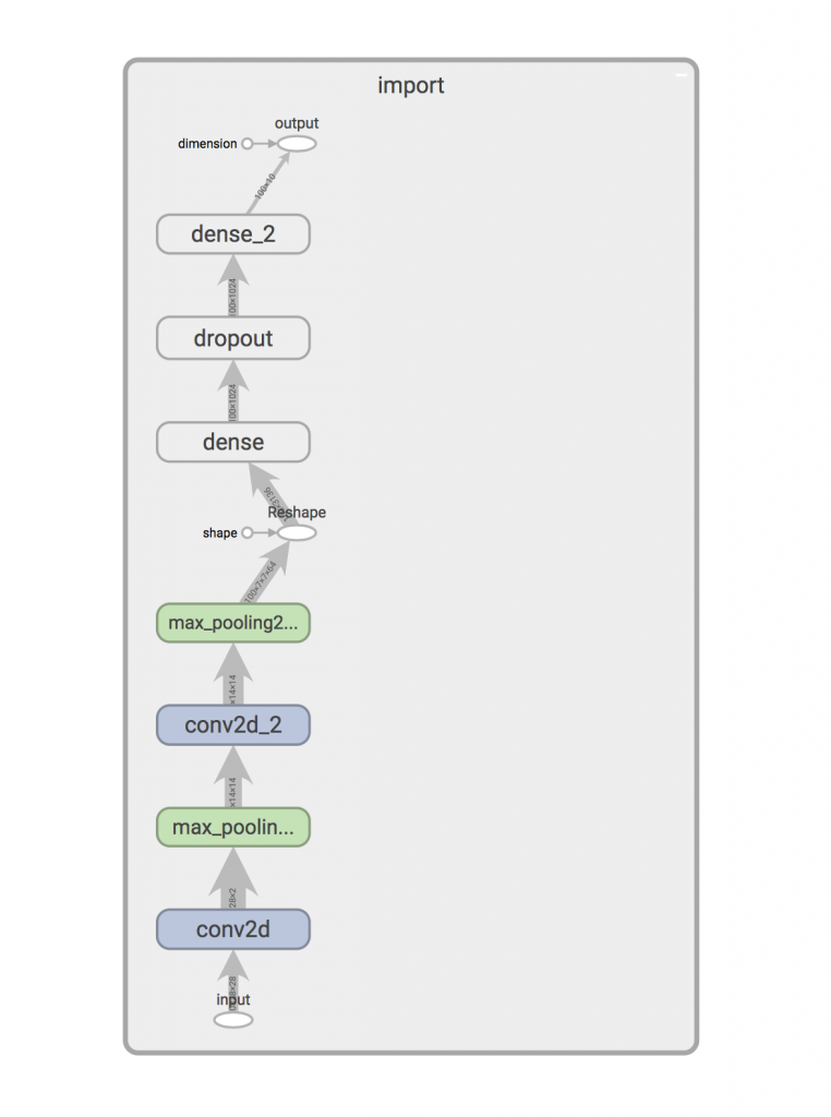
If you want to visualize your optimized graph with TensorBoard, check out How to inspect pretrained TF model.
We are now ready to begin using this in an Android project.
Integrating into an Android App
Deploying a trained TensorFlow neural network model is a relatively task.
Adding the TensorFlow Mobile dependency
Add the TensorFlow Mobile dependency to the build.gradle in the app/ folder, then sync the project’s Gradle dependencies.
implementation "org.tensorflow:tensorflow-android:1.5.0"
The class we are going to use to interact with our model, provided by TensorFlow Mobile, is TensorFlowInferenceInterface. It provides several methods for loading our model, feeding new data to the network, running inference, and extracting a prediction.
Adding the model
Copy your optimized graph to your Android project. It should be copied to src/main/assets. TensorFlowInferenceInterface will load the model from this folder in it’s constructor.
Some architecture
Our app will allow the user to draw a number with their finger. We will convert their drawing into a bitmap and pass that to our neural network for prediction. Recognizing this, the very first thing I will do is create a Classifier interface.
interface Classifier { fun predict(input: IntArray): Int fun close() }I am choosing to create an interface so that I can easily create more than one implementation of a Classifier. One using TensorFlow Mobile and one using TensorFlow Lite (in Part 2).
Using TensorFlowInferenceInterface
As stated before TensorFlowInferenceInterface is how we will be interacting with our trained network.
Let’s implement our Classifier interface by writing TFMobileClassifier.
class TFMobileClassifier(context: Context, modelFilename: String, private val inputName: String, private val inputDimensions: Pair<Long , Long>, private val outputName: String, private val outputSize: Int) : Classifier { override predict(input: IntArray): Int { TODO() } override close() { TODO() }}Our TFMobileClassifier has a constructor with 6 arguments. The Context is used to access files via AssetManager. The remaining arguments specify our model file and input and output node specifications.
Instantiating a TFMobileClassifier.
val classifier: Classifier = TFMobileClassifier(this, modelFilename = "file:///android_asset/optimized_graph.pb", inputName = "input", inputDimensions = Pair(28, 28), outputName = "output", outputSize = 100)
Let’s create our TensorFlowInferenceInterface.
private val assetManager = context.assetManagerprivate val inferenceInterface = TensorFlowInferenceInterface(assetManager, modelFilename)
Now that we have have a TensorFlowInferenceInterface, let’s start using it by implementing predict().
override fun predict(input: FloatArray) { // 1) create an array to store our predictions val predictions = LongArray(100)// 2) feed our data into input layer of our neural network inferenceInterface.feed(inputName, floatInput, 1, inputDimensions.first, inputDimensions.second, 1)
// 3) run inference between the input and specified output nodes inferenceInterface.run(arrayOf(outputName))
// 4) fetch the predictions from the specified output node inferenceInterface.fetch(outputName, predictions)
// 5) tabulate our predictions and return the most probable return processPredictions(predictions)}
A few things to talk about here:
- Our output node emits 100 values, so we need to store them in an array that contains at least 100 elements
- Our input data array size must equal the value when you compute the total elements in a X * Y * Z array. For example, our neural network uses 28 x 28 monochrome images. Our dimensions are going to be: 28 x 28 x 1. This means our input data array should contain 784 values.
- When running inference, we need to specify the name of the output node where inference will end.
- After inference has completed, we will store our results in the 100 element predictions array. This particular neural network returns an array containing 100 predictions given the input data. Going back to our Python training script, we trained our network in with batch_size = 100. This means, even though we feed the neural network a single image, it will give us 100 predictions on what it thinks the user has drawn.
- Because we have 100 predictions, we need to count the occurrence of each prediction, then return the digit that was the predicted the most. We will use this value as our prediction.
Our implemented TFMobileClassifier.
package com.emuneee.tensorandflow.classifier
import android.content.Contextimport android.content.res.AssetManagerimport org.tensorflow.contrib.android.TensorFlowInferenceInterfaceimport timber.log.Timberimport java.util.*import kotlin.Comparator
/** * Created by evan on 2/28/18. */class TFMobileClassifier(context: Context, modelFilename: String, private val inputName: String, private val inputDimensions: <Long , Long>, private val outputName: String, private val outputSize: Int) : Classifier {private val assetManager: AssetManager = context.assets private val inferenceInterface = TensorFlowInferenceInterface(assetManager, modelFilename)
override fun predict(input: IntArray): Int { val floatInput = input.map { it.toFloat() } .toFloatArray() // 1) create an array to store our predictions val predictions = LongArray(outputSize)// 2) feed our data into input layer of our neural network inferenceInterface.feed(inputName, floatInput, 1, inputDimensions.first, inputDimensions.second, 1)
// 3) run inference between the input and output nodes inferenceInterface.run(arrayOf(outputName))
// 4) fetch the predictions from the specified output node inferenceInterface.fetch(outputName, predictions)
// 5) tabulate our predictions and return the most probable return processPredictions(predictions) }
private fun processPredictions(predictions: LongArray): Int { val counts = predictions.toTypedArray() .groupingBy { it } .eachCount() val predictionSet = TreeSet<Pair<Long, Int>> (Comparator<Pair<Long, Int>> { o1, o2 -> o2!!.second.compareTo(o1!!.second) }) counts.toList() .forEach { pair -> predictionSet.add(pair) } val pair = predictionSet.first() Timber.d("Selecting ${pair.first} @ ${(pair.second / 100.0) * 100}% confidence") return pair.first.toInt() } override fun close() { inferenceInterface.close() }}Using the Classifier
Now that we have implemented a Classifier, it’s time to build some UI that allows the user to submit data with their fingertips. For brevity’s sake, I’m going to pass over a lot of the pure Android concepts, like layouts, and click listeners, etc. Our user interface has 3 components:
- We have a custom CanvasView that allows the user to user their fingertips to draw on a Canvas. When the user has finished drawing on the CanvasView it will emit a bitmap that represents the user’s drawing via a CanvasView.DrawListener
- We’ll have an ImageView that resembles actual data submitted to the neural network.
- Finally, we’ll have a TextView that displays the prediction.
Before we continue, we will need to address an issue. We’ll need to convert the user input to data format that resembles an image from the MNIST dataset. This is critical because the closer the data resembles the original training data, the more accurate our predictions. The MNIST training data set is filled with 28×28 monochrome images where for a given pixel, the values range from 0 (white) to 255 (black).
Here is how we convert the bitmap from our CanvasView to a monochrome, 28×28 bitmap:
private fun toMonochrome(bitmap: Bitmap): Bitmap { // scale bitmap to 28 by 28 val scaled = Bitmap.createScaledBitmap(bitmap, 28, 28, false)// convert bitmap to monochrome val monochrome = Bitmap.createBitmap(28, 28, Bitmap.Config.ARGB_8888) val canvas = Canvas(monochrome) val ma = ColorMatrix() ma.setSaturation(0f) val paint = Paint() paint.colorFilter = ColorMatrixColorFilter(ma) canvas.drawBitmap(scaled, 0f, 0f, paint)
val width = monochrome.width val height = monochrome.height
val pixels = IntArray(width * height) monochrome.getPixels(pixels, 0, width, 0, 0, width, height)
// Iterate over height for (y in 0 until height) {for (x in 0 until width) { val pixel = monochrome.getPixel(x, y) val lowestBit = pixel and 0xffif (lowestBit < 128) { monochrome.setPixel(x, y, Color.BLACK) } else { monochrome.setPixel(x, y, Color.WHITE) } } } return monochrome}The output from toMonochrome() is used to give the user an idea of what the input to the neural network looks like. It’s also converted to a format suitable for inference:
private fun formatInput(bitmap: Bitmap): IntArray { val pixels = IntArray(bitmap.width * bitmap.height) var i = 0 for (y in 0 until bitmap.height) { for (x in 0 until bitmap.width) { pixels[i++] = if (bitmap.getPixel(x, y) == Color.BLACK) 255 else 0 } } return pixels}We do two things here. First we flatten our 28×28 bitmap into a 784 element integer array. Finally, we convert each pixel value to either 0 or 255 if the pixel value is white or black, respectively.
Our MainActivity.kt looks like:
package com.emuneee.tensorandflowimport android.graphics.*import android.support.v7.app.AppCompatActivityimport android.os.Bundleimport kotlinx.android.synthetic.main.activity_main.*import android.graphics.Bitmapimport com.emuneee.tensorandflow.classifier.Classifierimport com.emuneee.tensorandflow.classifier.TFMobileClassifierimport com.emuneee.tensorandflow.view.CanvasViewimport timber.log.Timberclass MainActivity : AppCompatActivity() { private val classifier: Classifier by lazy {TFMobileClassifier(this, modelFilename = "file:///android_asset/optimized_graph.pb", inputName = "input", inputDimensions = Pair(28, 28), outputName = "output", outputSize = 100)}override fun onCreate(savedInstanceState: Bundle?) { super.onCreate(savedInstanceState) setContentView(R.layout.activity_main) Timber.plant(Timber.DebugTree()) canvas.drawListener = object: CanvasView.DrawListener { override fun onNewBitmap(bitmap: Bitmap) { Thread(Runnable {// convert the drawing to a 28x28 monochrome image val monochrome = toMonochrome(bitmap) // set the nn input image runOnUiThread { scaledCanvas.setImageBitmap(monochrome) }// convert the data to something that resembles the MNIST training data set val inputData = toIntArray(monochrome) // predict val pred = classifier.predict(inputData) runOnUiThread { prediction.text = pred.toString() } }).start() } } } override fun onDestroy() { super.onDestroy() classifier.close() }/** * Converts a Bitmap to a 28 x 28 monochrome bitmap */private fun toMonochrome(bitmap: Bitmap): Bitmap { // scale bitmap to 28 by 28 val scaled = Bitmap.createScaledBitmap(bitmap, 28, 28, false) // convert bitmap to monochrome val monochrome = Bitmap.createBitmap(28, 28, Bitmap.Config.ARGB_8888) val canvas = Canvas(monochrome) val ma = ColorMatrix() ma.setSaturation(0f) val paint = Paint() paint.colorFilter = ColorMatrixColorFilter(ma) canvas.drawBitmap(scaled, 0f, 0f, paint) val width = monochrome.widthval height = monochrome.heightval pixels = IntArray(width * height) monochrome.getPixels(pixels, 0, width, 0, 0, width, height) for (y in 0 until height) { for (x in 0 until width) { val pixel = monochrome.getPixel(x, y) val lowestBit = pixel and 0xff if (lowestBit < 128) { monochrome.setPixel(x, y, Color.BLACK) } else { monochrome.setPixel(x, y, Color.WHITE) } } } return monochrome }/** * Converts a bitmap to a flattened integer array */private fun toIntArray(bitmap: Bitmap): IntArray { val pixels = IntArray(bitmap.width * bitmap.height) var i = 0 for (y in 0 until bitmap.height) { for (x in 0 until bitmap.width) { pixels[i++] = if (bitmap.getPixel(x, y) == Color.BLACK) 255 else 0 } } return pixels }}That’s it! We have trained a neural network to recognize handwritten digits using TensorFlow, then successfully deployed it via an Android app.
In Part 2, I am going to re-implement our Classifier interface using TensorFlow Lite, instead of TensorFlow Mobile. TensorFlow Lite is a more lightweight framework for doing inference on a mobile device. It can also make use of specialized Neural Network acceleration hardware on Android 8.1+ devices.
In the meantime, all code, scripts, and model can be accessed on GitHub.
Originally published at emuneee.com on March 8, 2018.
Tensor & Flow: Part 1, TensorFlow & Machine Learning on Android was originally published in Hacker Noon on Medium, where people are continuing the conversation by highlighting and responding to this story.
Publication date
Disclaimer
The views and opinions expressed in this article are solely those of the authors and do not reflect the views of Bitcoin Insider. Every investment and trading move involves risk - this is especially true for cryptocurrencies given their volatility. We strongly advise our readers to conduct their own research when making a decision.