Latest news about Bitcoin and all cryptocurrencies. Your daily crypto news habit.
It’s difficult to say how many digital photos people produce every year, but the total number is estimated as more than 1 trillion per year. That huge amount of photos mostly come from mobile phones and quite often these images are stored in JPEG format. Apart from that, many industrial cameras also generate jpegs in huge volumes. Image extension .jpg is the most frequent choice, and this is actually a default setting in many smart phones and cameras. Abbreviation JPEG means both image format and lossy compression algorithm which is utilized for image encoding and decoding.
JPEG means Joint Photographic Experts Group, which created the standard. The first draft of JPEG standard was released in 1992. JPEG standard specifies the codec, which defines how an image is compressed into a stream of bytes and decompressed back into the image. It is not brand new algorithm, but this is solid ground and very popular method to store compressed images. Let’s have a look why it could be a good solution and how it’s actually working.
JPEG image compression algorithm is always lossy, which means that we don’t store full data from an original image. This is not actually a problem — algorithm removes image detail which most of people just can’t see. That method is called “visually lossless compression” to emphasize that level of image qualilty losses could be really low. In most cases we can get compression ratio in the range of 10–12 times, which saves us a lot of HDD/SSD space.
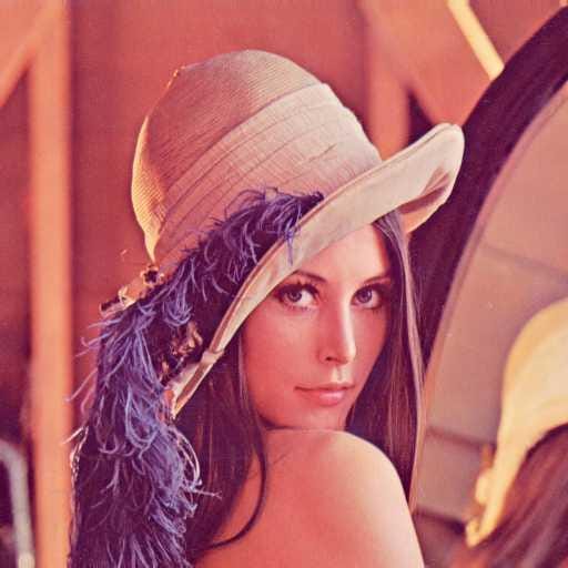
This is an example of extreme image quality losses with JPEG compression. You can see original Lena image in TIFF format (512x512, 24-bit, 769 kB, no compression) and the same image at JPEG format with quality compression coefficient 50%, subsampling 4:2:0, 24-bit, image size 23 kB. Can you see any noticeable difference at 100% scaling? Please note that this is extreme case with compression ratio ~33, though for visually lossless JPEG compression, recommended value is around 10–12.

JPEG compression and decompression used to be considered computationally intensive and slow. An idea about fast image compression was far from being true. Since then, new hardware and new approaches for parallel programming made JPEG fast, reliable and widespread.
General approach to image compression implies the following stages
- Color transform from RGB to YCbCr together with shift
- Sub-sampling and partitioning
- Transform to frequency domain
- Removal of high frequency detail from the image
- Reordering for better compression
- Removal of zeros series
- Lossless entropy coding to remove some more extra data
- Final packing
Color transform from RGB to YCbCr
That transform is based on our physiological experience. Human visual system can perceive minor changes of brightness, though it’s far less responsive to changes of color (chroma components of the image) for the regions with the same brightness. That’s why we can apply stronger compression to chroma to get less image size of compressed image. We take RGB image and convert it to luma/chroma representation in order to separate luma from chroma and to process them separately.
Luma is usually called Y (intensity, brightness) and chroma components are called Cb and Cr (these are actually differences Cb = B — Y and Cr = R — Y). That transform is done at the same time with data shift to prepare data to processing stage which is called DCT (discrete cosine transform).
Subsampling and partitioning
As soon as we can consider chroma components to be less important than luma, we can decrease the total number of chroma pixels. For example, we can average chroma in horizontal or vertical direction. At the most extreme case we can average 4 neighbor chroma values in the rectangle 2x2 to get just one new value. That mode is called 4:2:0 and this is the most popular choice for subsampling.
For further processing we divide the whole image into blocks 8x8 for luma and chroma. That partitioning scheme let us process each block independently, though we will have to remember coordinates of each block which are essential at image decoding.
DCT: Discrete Cosine Transform
DCT is a Fourier-related transform which is similar to the Discrete Fourier Transform (DFT), but using only real numbers. You can get more info at Wiki. Actually we apply that 2D transform to each block 8x8 of our image. The main idea is to get other data representation and to move from spatial to frequency domain. The result of DCT is data array in frequency domain and this is very clever step to work further not directly with luma and chroma, but with frequencies of luma and chroma from our image. Big objects on the image are considered to be low-frequency data, though small/tiny objects are considered to be high frequency elements.
In the new block 8x8 the upper left element is called DC (this is average value for all pixels from the original block), and all other elements are called AC. If we compose a new image from DC elements of each block, we get original image with reduced resolution. New width and height will be 1/8 from the original image. This is just an illustration of how DCT is working and what’s DC and AC.
It could sound strange, but at this step we don’t have any data reduction. Not at all. On the contrary, after DCT we get more data in comparison with data size on the previous step, but still, this is very important action. New representation soon will let us to achieve strong compression, but not right now. We do need some patience and it will be rewarded shortly.
Quantization and reordering
We’ve come to the point where we have to introduce some data losses. That stage is called quantization. At first, we create a special quantization matrix 8x8 with coefficients. At upper left part of the matrix these coefficients are equal to 1 or more, but towards lower right part they are getting bigger. Quantization means division of each value from 8x8 block to corresponding coefficient from quantization matrix.
After such a division and rounding, we get reduced values for each 8x8 block and the most important issue here is that we get many zeros for values which are close to right bottom part of the block. Quite often we can see some areas of the block which are filled with zeros. That is exactly what we hoped to get — series of zeros. This is the way how quantization detects high frequency elements to be discarded.
For further processing we apply so-called Zig-Zag algorithm to create linear array of values from the block. This is done via zigzag-like path when we start to move from upper left corner of the block and go to the right bottom corner. After such reordering we get series of values for each block 8x8. We will not work with blocks now, we will work with these reordered data.
After quantization we not only have less data, we’ve introduced some losses to original image. Most losses at JPEG compression algorithm comes here. That’s why the choice of quantization matrix is the key to get acceptable image quality of compressed image. JPEG standard doesn’t define such a matrix and many camera and software manufacturers apply lots of efforts to develop the best possible solution.
DC coding
Starting from that point we will process DC and AC elements separately. We start from delta coding for DC. We just take the first value from each block (this is DC component) and store the difference with DC value from previous block. This is very simple and straightforward. The thumbnail, which is composed from DC components, could be used as downsampled version of the original image.
RLE: Run Length Encoding
Starting from here, we will work with AC elements only and we remember that each block consists of 63 such values. Actually, we’ve come to the point where we finally can do data reduction. In each set of AC elements we can see series of zeros and now we can substitute them with some short codes which could store the same information. This is lossless algorithm and we don’t introduce any image losses here.
RLE method transforms sequence of values to sequence of pairs. The first element of the pair is called symbol, the second element of the pair is non zero value. For each series we code in the symbol the number of preceding zeroes and bit length of non-zero value. The idea of RLE is to store at just one value the number or consecutive zeros which we see before the next non-zero value from AC data. Here we have great data reduction and this is lossless transform! This is the way to shrink all series of zeros that we have among AC elements. But that is not all, we can get some more compression.
Huffman coding
That lossless compression algorithm is named after Huffman which was the inventor of that method. It’s also called entropy coding algorithm and here it’s applied to get better compression after RLE.
The idea of that algorithm is to compare all codes that we get after RLE and to choose the shortest representation with less bits for those codes which occurred more frequently. At Huffman stage we compute frequency of each symbol and create optimal bit code for each one. We will not get into more detail here, you can see full info at Wiki.
Final packing
Having finished with compression, we need to pack compressed data from all blocks, to add correct header for jpg, to set file name, and to store compressed file to HDD.
Each photo camera and smart phone does pretty much the same. We just had a look how it goes several billion times every day worldwide.
Tips and tricks
JPEG algorithm was created to compress real photographic images. It’s not good at artificial image compression, for example for images with text. If we try to compress such an artificial image with JPEG, the result is not bad, but that compression algorithm just wasn’t created for such a task.
Standard JPEG compression, which is based on DCT, can’t be lossless by definition. Even if we define compression quality to be 100% (which means no quantization), we still get some minor losses due to Color Transform and DCT, because after DCT we get float values which have to be converted to integer values, so we apply rounding and this is lossy operation. Please note that Lossless JPEG exists, but this is totally different algorithm, though with the same name.
When your software is asking you to save your image to JPEG, please note that there are many ways to define quality parameter, so suggested value could differ from your expectations quite a lot. Usually we utilize JPEG compression quality parameter which is in the range of 0–100%, but for real life it’s not less than 50%. Visually lossless JPEG compression is considered to be the case for quality 90% and more. To check it visually, you can try to discover slight rectangle borders at 100% zoom. If you don’t see them, it means that your compression is visually lossless for you at your viewing conditions, which is good.
JPEG standard allows so called restart markers which are built in jpeg bytestream and they are intended to offer much faster JPEG decompression. Nevertheless, most of cameras and software produce jpeg images without restart markers. You can check the number of restart markers in your jpegs with JpegSnoop software. Jpegtran utility can help you to insert desired number of restart markers into your jpeg images.
Some software manufacturers utilize their own units for compression quality like “jpg for web” or “quality level from 1 to 12”, so you need to be prepared to check that. The best way to prove such a compliance could be JpegSnoop software which can show you real value of compression quality for luma and chroma in standard units together with quantization matrices for luma and chroma.
If you need to do JPEG compression or decompression by yourself with any software, please bear in mind the following tools and libraries:
- JpegSnoop — very useful software to check what’s inside your jpeg images, including all meta tags and internal parameters: https://github.com/ImpulseAdventure/JPEGsnoop
- jpegtran — cross-platform tool for JPEG compression and decompression on CPU. Not very fast, but with lots of options: http://jpegclub.org/jpegtran/
- libjpeg — cross-platform library for JPEG compression and decompression on CPU. Not very fast, but with lots of options: http://libjpeg.sourceforge.net/
- Libjpeg-turbo — very fast library for JPEG encoding on CPU: http://libjpeg-turbo.org
- Fast image compression on CUDA (the fastest solution for JPEG encoder and decoder on GPU): https://www.fastcompression.com/
- FFmpeg — cross-platform solution to create video from your jpeg series on CPU: https://ffmpeg.zeranoe.com/builds/

Why Do We Need JPEG Compression and How It’s Technically Working? was originally published in Hacker Noon on Medium, where people are continuing the conversation by highlighting and responding to this story.
Publication date
Disclaimer
The views and opinions expressed in this article are solely those of the authors and do not reflect the views of Bitcoin Insider. Every investment and trading move involves risk - this is especially true for cryptocurrencies given their volatility. We strongly advise our readers to conduct their own research when making a decision.