Latest news about Bitcoin and all cryptocurrencies. Your daily crypto news habit.
A use-case and walkthrough of how we used the Gatsiva API to evaluate a proposed trading strategy for 0x (ZRX).
 Photo by Ylanite Koppens from Pexels
At Gatsiva, we’ve been applying machine learning to markets for over 15 years with equities, forex, and most recently, cryptocurrencies. We provide an analysis API that helps cryptocurrency traders become more confident in their trades, especially when using technical indicators to determine buy or sell signals.
In this article we show how this API was used to gain more confidence in trading approach, utilizing a recent case-study helping one of our collaborators evaluate a trading idea around 0x (ZRX).
The Proposed Strategy
A collaborator on our platform recently floated the idea: What if one could use slope of MACD Histogram to attempt to predict shifts in price before they occur? Would this provide advance insight for price declines or price increases? In particular, would this strategy work well for the coin in question — 0x (ZRX) priced in BTC?
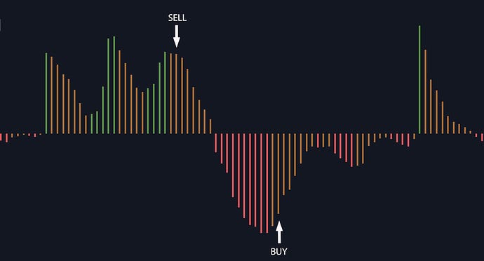 Illustration of MACD Histogram Slope Crossover Strategy
The first step was to design the condition that would capture these signals accurately. Utilizing Gatsiva’s natural language for condition definition we helped this user specify the proper condition to define the strategy. In this particular case, the pair of rules were easily defined as follows:
Rule 1 (Short): macd histogram(12,26,9) > 0 and slope of macd histogram(12,26,9) over 1 period crosses below 0Rule 2 (Long): macd histogram(12,26,9) < 0 and slope of macd histogram(12,26,9) over 1 period crosses above 0
The second step was to analyze the return profile of conditions. Utilizing our API, we can easily bring in the return data needed to generate the following visualizations, one for each condition we’ve defined.
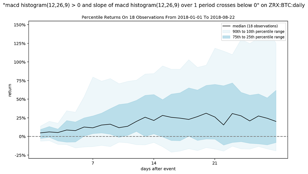 Rule 1 (SHORT) Percentile Return Profile
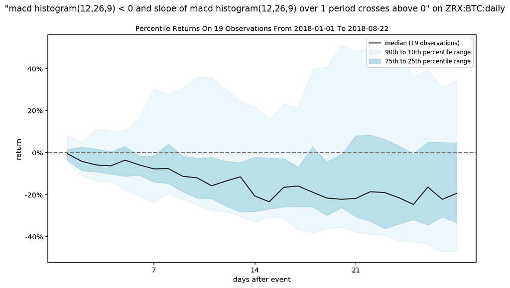 Rule 2 (LONG) Percentile Return Profile
These visualizations show the distribution of returns over the number of periods after an event occurs. It’s a way of summarizing historical data to illustrate “what happened next”.
For a more detailed explanation of these confidence band charts and how to create them, take a look at our prior articles: Trading Cryptocurrency with Confidence Bands and Gatsiva + Python: Visualizing Bitcoin Corrections. To jump right into code, you can also check out our open source Python Notebooks.
Interestingly, we can see here that these rules seem to be pretty well paired. One has a positive orientation while the other has a negative orientation. However, what is perhaps MORE interesting is that we notice that these rules seemed to indicate the opposite approach of what we initially thought.
Usually MACD histogram being positive and sloping downward is a sign of overbought scenarios. Likewise, the opposite being a sign of an oversold scenario. But in this case, the return profile indicates precisely the opposite.
When the MACD Histogram was positive and the slope shifted downward (Rule 1), returns were often higher in the next few days indicating this would be a better LONG rule than a SHORT rule. Similarly, when MACD Histogram was negative and the slope shifted upward, returns continued to be negative — indicating that this was a better SHORT rule than a LONG rule.
This is the first superpower of the Gatsiva API — the ability to show an analyst real returns after an event. This can help easily support or quickly debunk notions of “this should just work” well before forming a trading strategy.
Simulating Trades
Next was the trade simulation. At Gatsiva, we’ve built an internal trade simulator that allows us to utilize 5-minute interval data from Binance to simulate trades from these signals.
Since our main data source is Cryptocompare, utilizing a separate data source to simulate trades is necessary to minimize data snooping bias as well as a way to get a more realistic trade entry experience by utilizing more granular time slices.
We assumed a starting portfolio of 10 BTC, allowing a maximum of 5 simultaneous open positions each with 20% available capital applied to the new position. Lastly, we assumed a commission cost of 0.1%.
Because our actual signals are delayed slightly (from the time data is available to the time the signal is processed and sent via our engine) we need to also model this time delay in our simulation. For this we give ourselves a generous 20 minute delay. In total, we apply the following trade entry rules to make sure that our entry was realistic.
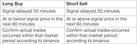 Trade Entry Rules
The exit criteria was simple: Apply a 15% trailing stop and a 20% profit target. We also update the trailing stop as profitability emerges, and hold for a maximum of 72 hours. If we reach the maximum hold, we sell at the average of the open, close, and low observed during the 5 minute tick interval. These exit rules are applied to both LONG and SHORT positions.
Note: This equates to a maximum of 3% loss of total value on any 1 trade when combined with our position sizes (15% trailing stop x 20% overall position size).
Lastly, we chose the data from 2018–01–01 to 2018–08–09 (date of the analyis). This was to ensure some history available from 0x before beginning technical analysis.
The Results
The overall results for 0x (ZRX) were impressive and shown in the tables and charts below. We were able to realistically enter 78% of the trades generated from our signals and make over 14% with commissions included. The lowest our simulated portfolio ever reached during this time period was 9.81 BTC (or approximately -1.9% of our original starting capital).
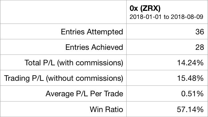 Table of Simulation Results
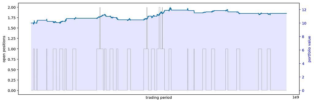 Portfolio Value and Open Positions Over Time
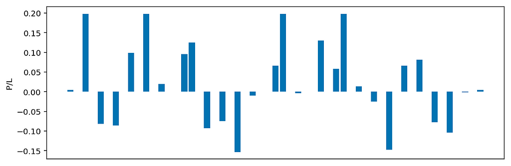 P/L of Each Trade
For the detailed list of simulated trades and timestamps, please take a look at this gist on Github.
Criticisms
From these results, we of course can anticipate many criticisms, and some of them will be fair. To head of two of them in particular — time-frame selection and coin selection — we offer the following:
It is possible that our timeframe selected skews the results. It is useful to note that during this simulation period of 2018–01–01 to 2018–08–09, 0x (ZRX) had an overall price increase in BTC of nearly 132%. We must recognize that these results are just “lucky” in that we’re benefiting from the initial run up.
In order to test this, we select a time period that most close matches the closing price at 2018–08–09 and find that 2018–02–02 would be a good starting point to test that theory. Below is a comparison of selecting a relative “flat” return period also with positive results.
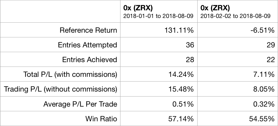 Comparison of Simulation Results to Flat Time Period
In the table above, we can see that even in a time period where the return was slightly negative, this strategy produced positive results.
Another fair criticism is the selection of 0x (ZRX) for this simulation compared to other coins. However, remember that before entering this strategy, we validated our assumptions on the viability of this MACD Histogram Slope Crossover signals as applied to 0x (ZRX).
That said, it is interesting to note that similar results can be observed for Ethereum (ETH), Ethereum Classic (ETC), and Litecoin (LTC) over the same time period.
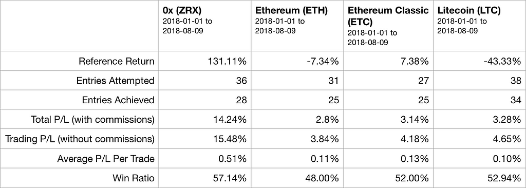 Comparison of Simulation Results to Other Coins
In the above table we can clearly see that for ETH, ETC, and LTC we get positive results in a mixed environment by coin. Ethereum and Ethereum Classic were relatively flat during this time period, but the simulation outperformed in both scenarios. Litecoin lost over 43% of its value during this time period, but the MACD Histogram Crossover strategy actually made 3.28% after commissions in this environment.
Making marginal gains in a down market … we’ll take it over losing money any day.
Putting This Into Action
So what do we now do with this information? After these results, these two conditions have been added to our Insight Engine and are now being constantly re-evaluated in realtime as new market data is produced. Any relevant signals based on our models are then fed to our collaborators as a signal available for discussion on our platform.
It is important to note that this strategy will not work for all coins in all cases. This becomes the second superpower of the Gatsiva platform — the ability to continually track and update which signals work for which coins. Carefully applied and validated with statistical tools in realtime, such signals can be a powerful addition to one’s trading signal arsenal.
Interested in Tools For Your Own Strategies?
Come and visit us at gatsiva.com, sign up for our collaboration platform, or better yet, take a look at the documentation to our API and get building your own strategies. We’re extending our API based on collaborator feedback.
Finally, if you like what you just read: Feel free to bookmark this article, clap, or leave a comment! It helps us help more people!

How to Validate a Crypto Trading Strategy was originally published in Hacker Noon on Medium, where people are continuing the conversation by highlighting and responding to this story.
Publication date
Disclaimer
The views and opinions expressed in this article are solely those of the authors and do not reflect the views of Bitcoin Insider. Every investment and trading move involves risk - this is especially true for cryptocurrencies given their volatility. We strongly advise our readers to conduct their own research when making a decision.